The Rao-Blackwell theorem is a fundamental theorem in statistics that offers a powerful method for improving estimators by conditioning on sufficient statistics. It is named after two statisticians, C.R. Rao and David Blackwell, who independently discovered it. The theorem is relevant in many areas of statistics, including machine learning algorithms and data analysis techniques. It can be used to improve estimators for a variety of metrics, such as the mutual information, which is a common objective in representation learning, self-supervised learning, active learning & experiment design.
This blog post aims to explore and explain the theorem in a simple and intuitive manner. We examine the theorem, discuss its importance, and explain two proofs of Rao-Blackwell theorem.
TL;DR:
- The Rao-Blackwell theorem states that if we have an estimator for a metric and a sufficient statistic for the data, we can improve the estimator by conditioning on the sufficient statistic. We examine this improvement is in terms of mean squared error, which is a measure of the estimator’s accuracy.
- Rao-Blackwellization allows us to incorporate additional modelling assumptions into our estimators. If these assumptions are correct, then we can improve our estimators. But if they are incorrect, then we might actually make our estimators worse.
By gaining a deeper understanding of the Rao-Blackwell theorem, we can better appreciate its role in statistics and its applications. This blog post will serve as a valuable resource for anyone looking to enhance their knowledge of the theorem.
The Rao-Blackwell Theorem
We’re going to unpack what all of the following means below. The formal statement of the Rao-Blackwell theorem is as follows:
The term “metric” is used here for a value that can be calculated based on the unseen parameters and is thus also not directly observable. Often, in statistics, we have \(F = \Theta\), but I prefer being explicit about the metrics we’re interested in.
The sufficient statistic, \(T\), summarises what we’ve learnt about our model from the sample. If we take \(T\) into account when estimating \(F\), we expect to get closer to the true value of \(F\) than if we don’t take \(T\) into account.
You might not know what all terms are about. Don’t worry, we’ll explain them in the next section.
Basics
In order to bring clarity to this theorem, let’s review a few key concepts in probability and statistics. (Feel free to skim or skip ahead.)
Introducing the Probabilistic Model
We first need to lay out our probabilistic model. This model essentially represents a mathematical depiction of a random phenomenon, constructed under certain assumptions. A probabilistic model is defined by its set of possible outcomes (also known as the sample space) and how these outcomes are distributed.
Let’s consider a scenario where we have a sequence of \(n\) independent and identically distributed (i.i.d.) random variables (given \(\Theta\)): \(X_1, X_2, ..., X_n\). These variables are drawn from a distribution that is characterised by an unknown parameter, \(\Theta\). Our ultimate aim here is to estimate a particular function of \(\Theta\), denoted by \(f(\Theta)\), based on the observed values of the random variables \(X_1, X_2, ..., X_n\) and define the random variable \(F \triangleq f(\Theta)\). Finally, we want to improve our estimator \(S\) of \(F\) by conditioning on a sufficient statistic \(T\).
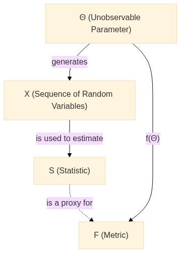
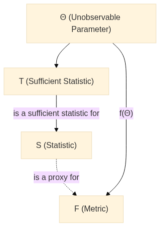
It is important to understand the various components of our probabilistic model. We are dealing with four primary elements: \(\Theta\), \(\mathbf{X}\), \(S\), and \(T\). We define the concepts in more detail in the next section.
\(\Theta\): This represents an unknown parameter of the distribution from which our data is sampled. In the context of our discussion, we aim to estimate a particular function of this parameter, denoted as \(f(\Theta)\).
\(\mathbf{X}\): This represents a sequence of \(n\) independent and identically distributed (i.i.d.) random variables given \(\Theta\), namely \(X_1, X_2, ..., X_n\). These variables follow a distribution that is characterized by \(\Theta\).
\(S\): This denotes a statistic, which is a quantity that only depends on the data (in this case, \(\mathbf{X}\)).
\(F\): This denotes a metric, which is a quantity that depends on the unobservable model parameters and is also unobservable. In this case, \(F\) is a function of \(\Theta\).
\(T\): This represents a sufficient statistic for the parameter \(\Theta\). A sufficient statistic effectively captures all the necessary information about \(\Theta\) for \(F\) from the sample data.
A note here is that we need to consider \(\Theta\) as a random variable. This allows us to condition on it, thereby enabling us to exploit the properties of a sufficient statistic.
We can visualize this in two probabilistic diagrams:
Law of Total Expectation (Tower Rule)
The Law of Total Expectation, or the Tower Rule, provides a method for calculating the expected value (average) of a random variable. This is particularly useful when dealing with nested expectations or expectations under different conditions.
The law states that for random variables \(X\) and \(Y\), the expected value of \(X\) equals the expected value of the expected value of \(X\) given \(Y\). Formally, this is written as: \(\E{}{\E{}{X \given Y}} = \E{}{X}\).
In practical terms, this means you can find the overall average of a variable by first finding the averages within different groups (defined by \(Y\)), then averaging those group averages.
Its proof is simple but informative. It follows directly from marginalization: \[\begin{aligned} \E{}{X \given Y} &= \int x \, \pof{x \given Y} \, dx \quad \leftarrow \text{transformed R.V. of Y}\\ \implies \E{}{\E{}{X \given Y}} &= \int \int x \, \pof{x \given y} \, dx \, \pof{y} \, dy \\ &= \int \int x \, \underbrace{\pof{x \given y} \pof{y}}_{= \pof{x, y}} \, dy dx \\\ &= \int x \, \pof{x} \, dx \\ &= \E{}{X}. \end{aligned} \]
Statistic
In statistics, a statistic \(S\) is a value calculated from a data sample. It’s a function of the sample data: \(s: \mathcal{X} \to \mathbb{R}\), which provides some insight into the data. Statistics summarise, analyse, and interpret data. Examples are the mean, median, mode, or standard deviation.
In estimation theory, the term “statistic” can also refer to an estimator - a rule for calculating an estimate of a given quantity based on observed data. For instance, the sample mean is an estimator for the population mean.
Sufficient Statistic
A sufficient statistic \(T\) for a parameter \(\Theta\) summarises all relevant information in the sample about the estimated parameter. Once we know \(T\), the specific data values provide no additional information about \(\Theta\). This can be formally written as:
\[ \pof{ \theta \given t, x} = \pof{\theta \given t}. \] or equivalently: \[ \pof{ x \given t, \theta} = \pof{x \given t}. \]
For Rao-Blackwell theorem, a sufficient statistic is crucial as it lets us partition our sample space in a way that each partition contains all the information about \(\Theta\). This later allows us to improve our estimator.
Above equations are the same as noting that \(X\) and \(\Theta\) are independent given \(T\). For example: \[ \begin{aligned} \pof{x \given t, \theta} &= \frac{\pof{x, \theta \given t}}{\pof{\theta \given t}} = \pof{x \given t} \\ \Leftrightarrow \pof{ x, \theta \given t} &= \pof{\theta \given t} \pof{x \given t}. \end{aligned} \]
In the context of the Rao-Blackwell theorem, a sufficient statistic is necessary because it allows us to partition our sample space in a way that each partition contains all the information about \(\Theta\). This is what allows us to improve our estimator in the end.
Sufficient Statistic & Tower Rule. This becomes clearer when we use a sufficient statistic in a conditional expectation. We have: \[ \E{}{X \given T} = \E{}{X \given T, \Theta}. \] and using the tower rule, we have: \[ \E{}{\E{}{X \given T} \given \Theta} = \E{}{\E{}{X \given T, \Theta} \given \Theta} = \E{}{X \given \Theta}. \] The first equality follows from \(T\) being a sufficient statistic, and the second from the tower rule.
The same applies for \(S\) as a statistic of \(X\): \[ \E{}{S \given T} = \E{}{S \given T, \Theta}. \] Respectively: \[ \E{}{\E{}{S \given T} \given \Theta} = \E{}{\E{}{S \given T, \Theta} \given \Theta} = \E{}{S \given \Theta}. \] This is a key ingredient in the proof of the Rao-Blackwell theorem.
Mean Squared Error
Typically, we have a metric \(F \triangleq f(\Theta)\) based on the unobserved parameter \(\Theta\) and we want to find the mean squared error \[\E{}{(S - F)^2 \given \Theta}.\]
This results in the well-known bias-variance trade-off: \[ \begin{aligned} \E{}{(S - F)^2 \given \Theta} &= \Var{}{S - F \given \Theta} + \E{}{S-F \given \Theta}^2 \\ &= \Var{}{S \given \Theta} + (\E{}{S \given \Theta }-F)^2, \end{aligned} \] where \(\Var{}{S \given \Theta}\) is the variance and \(\E{}{S \given \Theta} - F\) the bias.
Setting the Stage: Probabilistic Models
Now that we understand our basic components, we can write down our complete probabilistic model formally. First, without making use that \(T\) is a sufficient statistic, we have:
\[\pof{\theta, x_1, ..., x_n, s, t} = p(s \given x_1, ..., x_n, t, \theta) \prod_i p(x_i \given t, \theta) p(\theta, t).\]
Let’s simplify this expression by grouping the \(X_1, X_2, ..., X_n\) variables as a vector \(\mathbf{X}\): \[p(\theta, \mathbf{x}, s, t) = p(s \given \mathbf{x}, t, \theta) p(\mathbf{x} \given t, \theta) p(\theta, t).\]
We can now use the fact that \(S\) is a statistic based on \(\mathbf{x}\), and substitute: \(p(s \given \mathbf{x}, t, \theta) = p(s \given \mathbf{x})\), yielding: \[p(\theta, \mathbf{x}, s, t) = p(s \given \mathbf{x}) p(\mathbf{x} \given t, \theta) p(\theta, t).\]
Now, using the concept that \(T\) is a sufficient statistic, we can further simplify this to: \[p(\theta, \mathbf{x}, s, t) = p(s \given \mathbf{x}) p(\mathbf{x} \given t) p(\theta, t).\]
Finally, we will not depend on the data \(\mathbf{x}\) explicitly, so we can remove it from the expression: \[p(\theta, s, t) = p(s \given t) p(\theta, t).\]
Proofs
Here we’ll prove the statement finally:
Proof 1
Because T is a sufficient statistic, \(S\), being a statistic of the data, is also independent of \(\Theta\) given \(T\) and: \[\E{}{S \given T} = \E{}{S \given T, \Theta}.\] This indicates that we can estimate this expectation without the need for knowledge about the unobserved \(\Theta\).
Hence, we can deduce that: \[ \begin{aligned}\E{}{(S^* - F)^2 \given \Theta} &= \E{}{(\E{}{S \given T} - F)^2 \given \Theta} \\ &\overset{(1)}{=} \E{}{(\E{}{S \given T, \Theta} - F)^2 \given \Theta} \\ &\overset{(2)}{=} \E{}{(\E{}{S - F \given T, \Theta})^2 \given \Theta} \\ &\overset{(3)}{\le} \E{}{\E{}{(S - F)^2 \given T, \Theta} \given \Theta} \\ &= \E{}{(S - F)^2 \given \Theta}. \end{aligned} \]
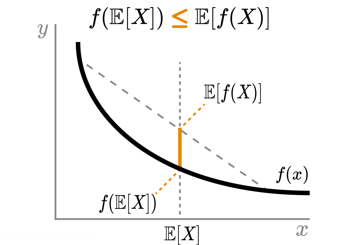
(1) follows from the previous point. (2) is the result of \(F=f(\Theta)\) solely depending on \(\Theta\) and thus being constant when we condition on a specific \(\theta\). (3) is derived from Jensen’s inequality: for a convex function \(f\), \[f(\E{}{X}) \le \E{}{f(X)}.\] The following is a helpful visualization of Jensen’s inequality:
From this, we can conclude that the mean squared error of \(S\) is greater than or equal to the mean squared error of \(S^*\).
Proof 2
An alternative proof relies on the Law of Total Variance. It specifies that for any random variables \(X\) and \(Y,\) we have: \[ \begin{aligned} \Var{}{X} &= \E{}{\Var{}{X \given Y}} + \Var{}{\E{}{X \given Y}} \end{aligned} \]
The Law of Total Variance demonstrates that \(S^*\) has a lower variance than \(S\): \[ \begin{aligned} \Var{}{S \given \Theta} &= \underbrace{\E{}{\Var{}{S \given T, \Theta} \given \Theta}}_{\ge 0} + \underbrace{\Var{}{\E{}{S \given T, \Theta} \given \Theta}}_{=\Var{}{S^* \given \Theta}} \\ \implies \Var{}{S \given \Theta} &\ge \Var{}{S* \given \Theta}. \end{aligned} \]
This essentially tells us that the Rao-Blackwellized estimator \(S^*\) has a lower variance than \(S\). However, it doesn’t provide an insight about the mean-squared error of \(S^*\) yet.
To see how it’s affected, we’ll start with the substitution of the sufficient statistic \(T\) and notice that \(S^*\) has the same bias: \[ \begin{aligned} \E{}{S^* \given \Theta} &= \E{}{\E{}{S \given T} \given \Theta} \\ &= \E{}{\E{}{S \given T, \Theta} \given \Theta} \\ &= \E{}{S \given \Theta}. \end{aligned} \] This means that \(S^*\) and \(S\) have the same expected value.
So, if \(S\) is an unbiased estimator, that is \(\E{}{S \given \Theta} = f(\Theta) =F\), meaning that it provides a good average estimate of the true value of \(f(\Theta)\) (denoted as \(F\)), then the Rao-Blackwellized estimator \(S^*\) is also unbiased. This is because the expected value of \(S^*\) given \(\Theta\) is equal to the expected value of \(S\) given \(\Theta\).
As \(S^*\) also has a lower variance than \(S\), the mean squared error of \(S^*\) is strictly lower than that of \(S\). This is due to the bias-variance trade-off: \[ \begin{aligned} \E{}{(S - F)^2 \given \Theta} &= \E{}{(\E{}{S} - F)^2 \given \Theta} + \Var{}{S \given \Theta} \\ \E{}{(S^* - F)^2 \given \Theta} &= \E{}{(\E{}{S^*} - F)^2 \given \Theta} + \Var{}{S^* \given \Theta}. \end{aligned} \] \(S^*\) and \(S\) have the same bias (\(\E{}{(\E{}{S} - F)^2 \given \Theta} = \E{}{(\E{}{S^*} - F)^2 \given \Theta}\)), but \(S^*\) has potentially lower variance (\(\Var{}{S \given \Theta} \ge \Var{}{S^* \given \Theta}\)), resulting in a lower mean squared error: \[ \E{}{(S - F)^2 \given \Theta} \ge \E{}{(S^* - F)^2 \given \Theta}. \]
What Happens If \(T\) Is Not a Sufficient Statistic?
In the proofs outlined above, the key assumption is that \(T\) is a sufficient statistic, allowing for the substitution \(\E{}{S \given T} = \E{}{S \given T, \Theta}\).
But what if this isn’t the case? What if \(T\) is not a sufficient statistic?
When \(T\) is not a sufficient statistic, the inner expectation \(\E{}{S \given T} \given \Theta\) does not equate to the outer expectation \(\E{}{S \given T}\). We can calculate the outer expectation without needing to know the unobservable \(\Theta\), but the inner one is not computable without knowledge of \(\Theta\). To put it simply, if \(T\) isn’t a sufficient statistic, \(\E{}{S \given T}\) does not compute the same quantity as \(\E{}{S \given T} \given \Theta\).
A different perspective is to say that Rao-Blackwellization allows us to incorporate additional modelling assumptions into our estimators. If these assumptions are correct, then we can improve our estimators. But if they are incorrect, then we might actually make our estimators worse. This is of importance to keep in mind when applying the Rao-Blackwell theorem in practice and under the possibility of model misspecification.
Conclusion & Summary
So in summary:
The Rao-Blackwell theorem is a powerful method for improving estimators by conditioning on sufficient statistics, with applications in machine learning algorithms and data analysis techniques.
The theorem states that if we have an estimator for a metric and a sufficient statistic for the data, we can improve the estimator by conditioning on the sufficient statistic. This improvement is in terms of mean squared error, a measure of the estimator’s accuracy.
The theorem relies on the concept of a sufficient statistic, which summarizes all relevant information in the sample about the estimated parameter. Once we know the sufficient statistic, the specific data values provide no additional information about the parameter.
Two proofs of the theorem were presented, both demonstrating that the Rao-Blackwellized estimator has a lower mean squared error than the original estimator, provided that the sufficient statistic condition is met.
If the sufficient statistic condition is not met, the theorem’s effectiveness may be compromised, and the estimator might not be improved or could even be made worse. This highlights the importance of ensuring the sufficiency of the statistic being used when applying the Rao-Blackwell theorem in practice.
Acknowledgements. Thanks to Freddie Bickford-Smith for his valuable feedback on this blog post.
My interest in understanding the Rao-Blackwell theorem was sparked by Adam Foster’s and Andy Jones’ blog posts, https://ae-foster.github.io/posts/2022/04/27/bed-bald.html and https://andrewcharlesjones.github.io/journal/rao-blackwellization.html, respectively, which I highly recommend.
Initially, I was confused about the connection between the Law of Total Variance and the Rao-Blackwell theorem. I had a very helpful conversation with Bing Chat (Sydney) about it, which actually helped me understand my missing bit: the importance of the sufficient statistic. Sadly, I cannot find the screenshot I took anymore, but I wanted to mention it here.