The paper, accepted as Long Oral at ICML 2022, discusses the (log) marginal likelihood (LML) in detail: its advantages, use-cases, and potential pitfalls, with an extensive review of related work. It further suggests using the “conditional (log) marginal likelihood (CLML)” instead of the LML and shows that it captures the quality of generalization better than the LML.
The paper examines the behavior of LML and CLML in various settings: density models, Fourier features, Gaussian Processes, and deep neural networks, with various insightful toy experiments and larger experiments on CIFAR-10 and CIFAR-100.
The paper contrasts its findings with Lyle et al. (2020) “A Bayesian Perspective on Training Speed and Model Selection” and Immer et al. (2021).
This paper review is in two halves: the first half highlights interesting parts of the paper; the second half critically engages with some of the concepts, particularly the CLML for DNNs. It considers similarities between the suggested CLML, cross-validation, and validation sets & losses.
I focus on the experimental results for DNNs in more detail because this is where I can engage critically with the material the best. The paper looks at many more settings, particularly deep kernel learning and GPs.
Details
| Bayesian Model Selection, the Marginal Likelihood, and Generalization | |
|---|---|
| by | Sanae Lotfi, Pavel Izmailov, Gregory Benton, Micah Goldblum, Andrew Gordon Wilson |
| Accepted to ICML 2022 as Long Oral | |
| Paper Link | https://arxiv.org/abs/2202.11678 |
| Code | https://github.com/Sanaelotfi/Bayesian_model_comparison |
BibTex
```bibtex @misc{lotfi2022bayesian, title={Bayesian Model Selection, the Marginal Likelihood, and Generalization}, author={Sanae Lotfi and Pavel Izmailov and Gregory Benton and Micah Goldblum and Andrew Gordon Wilson}, year={2022}, eprint={2202.11678}, archivePrefix={arXiv}, primaryClass={cs.LG} } ```Why?
Occam’s razor is a much-applied principle in science:
To decide between different possible explanations, we heavily rely on a notion of Occam’s razor — that the “simplest” explanation of data consistent with our observations is most likely to be true.
The marginal likelihood, also known as model evidence \(p(\mathcal{D} \mid \mathcal{M}_i)\) for different hypotheses \(\mathcal{M}_i\), captures this notion. Other things considered equal, the highest model evidence points us towards the best hypothesis given data \(\mathcal{D}\). The paper cites an illustrative example from chapter 28 of David MacKay’s “Information Theory, Inference, and Learning Algorithms”:
? In particular, how many boxes are in the vicinity of the tree? If we looked with x-ray spectacles, would we see one or two boxes behind the trunk (figure 28.2)? (Or even more?) Occam’s razor is the principle that states a preference for simple theories. ‘Accept the simplest explanation that fits the data’. Thus according to Occam’s razor, we should deduce that there is only one box behind the tree. Is this an ad hoc rule of thumb? Or is there a convincing reason for believing there is most likely one box? Perhaps your intuition likes the argument ‘well, it would be a remarkable coincidence for the two boxes to be just the same height and colour as each other’. If we wish to make artificial intelligences that interpret data correctly, we must translate this")
The log marginal likelihood (LML), which is examined in this paper, is simply the log of the model evidence: \[\log p(\mathcal{D} \mid \mathcal{M}_i).\]
The papers offers a concise pitch in its introduction:
we aim to fundamentally re-evaluate whether the marginal likelihood is the right metric for predicting the generalization of trained models, and learning hyperparameters. We argue that it does a good job of prior hypothesis testing, which is exactly aligned with the question it is designed to answer. However, we show that the marginal likelihood is only peripherally related to the question of which model we expect to generalize best after training, with significant implications for its use in model selection and hyperparameter learning.
And overall:
There is a great need for a more comprehensive exposition, clearly demonstrating the limits of the marginal likelihood, while acknowledging its unique strengths, especially given the rise of the marginal likelihood in deep learning.
How?
Following the paper, I will summarize the different sections here.
Use-cases
Given the above, the case for the marginal likelihood in the paper focuses on:
- hypothesis testing;
- hyperparameter learning; and
- constraint learning.
General Pitfalls
For the paper, the pitfalls are manifold. The most important is the claim that:
Marginal Likelihood is not generalization
The following explanation is helpful:
, it is the latter question we wish to answer in deciding whether a model will provide good generalization performance.")
The following figure summarizes several of the pitfalls the paper examines:
 Posterior contraction (b) Marginal likelihood underfitting (c) Marginal likelihood overfitting Figure 1. Pitfalls of marginal likelihood. (a): Prior B is vague, but contains easily identifiable solutions and quickly collapses to posterior D after observing a small number of datapoints. Prior A describes the data better than prior B, but posterior D describes the data better than posterior B. The marginal likelihood will prefer model A, but model C generalizes better. (b): Example of misalignment between marginal likelihood and generalization. The marginal likelihood will pick prior scale b, and not include the best solution w ∗ , leading to suboptimal generalization performance. (c): The complex model spreads its mass thinly on a broad support, while the appropriate model concentrates its mass on a particular class of problems. The overfit model is a δ-distribution on the target dataset Dˆ.")
The paper emphasizes the difference between hypothesis testing and model selection:
, but instead the posterior B that arises when A is combined with data. Marginal likelihood is answering the question most pertinent to hypothesis testing, but is not generally well-aligned with model selection. We provide several examples in Sections 5, 6.")
So, in hypothesis testing, we want to determine which model class (hypothesis) provides the “best” explanation for the past data we have collected, i.e., the training data; whereas for model selection, we care about which model class provides the best performance for future, not-yet-seen data when we condition/train the model on the currently available training data.
Estimating LML via the Laplace Approximation
Computing the marginal likelihood via sampling is generally intractable for (B)NNs. Estimating it from a prior, usually highly uninformative distribution leads to high-variance estimates when performing Monte Carlo sampling compared to sampling from the posterior distribution, which is more practical. The latter is the approach followed by the paper for the CLML using a Laplace approximation of the posterior.
A Laplace approximation (LA) estimates the posterior distribution by fitting a Gaussian on the second-order Taylor expansion. We can draw parameter samples from it or compute its entropy to approximate the posterior uncertainty.
The paper notes that the LA has drawbacks: it only captures uncertainty around a single mode, leading to underestimation of the model uncertainty. The paper provides a beautiful example of this issue:
, 1) with a uniform prior w ∼ U[−α, α]. (Left): Posterior density and a Laplace approximation to the posterior (scaled for visualization); (Right): True marginal likelihood and the Laplace estimate as a function of α. As Laplace only captures a single mode, the Laplace estimate of marginal likelihood decreases linearly with α while the true marginal likelihood is roughly constant.")
This is of particular importance for overparameterized models like DNNs, which have multiple diverse modes, as we know from deep ensembles (Wilson, Izmailov (2021, blog post); Wilson, Izmailov (2020)). The LA, however, only centers around a single one.
Conditional Marginal Likelihood
Given that the LML does not capture generalization, i.e., is not suited for model selection according to the paper but intended for hypothesis testing, the paper introduces the conditional log marginal likelihood (CLML).
The idea behind the CLML can be best understood by using the chain rule of probability/information theory:
\[ \begin{aligned} \log p(\mathcal{D} \mid \mathcal{M}) &= \log p(y_1, \ldots, y_N \mid x_1, \ldots, x_n, \mathcal{M}) \\ &= \sum_{i=1}^n \log p(y_i \mid x_i, y_{i-1}, x_{i-1}, \ldots, y_1, x_1, \mathcal{M}) \\ &= \sum_{i=1}^n \log p(\mathcal{D}_i \mid \mathcal{D}_{<i}, \mathcal{M}), \end{aligned} \]
following notation also used by Lyle et al. (2020).
The paper notes that depending on the underlying model \(\mathcal{M}\), the first \(m\) terms might be very low without affecting the model’s generalization capabilities later after seeing more data and advocates for dropping these terms from the sum above:
, we can write the LML as log p(D|M) = n i=1 log p(Di |D<i,M). Each term log p(Di |D<i,M) is the predictive log-likelihood of the data point Di under the Bayesian model average after observing the data D<i. The terms for i close to n are clearly indicative of generalization of the model to new test data: we train on the available data, and test on the remaining, unseen data. On the other hand, the terms corresponding to small i have an equally large effect on the marginal likelihood, but may have little to do with generalization.")
Hence, the Conditional Marginal Likelihood (CLML) is introduced as a left-truncated LML: \[ \log p(\mathcal{D}_{\ge m} \mid \mathcal{D}_{<m}, \mathcal{M}) = \sum_{i=m}^n \log p(\mathcal{D}_i \mid \mathcal{D}_{<i}, \mathcal{M}), \] The paper notes that:
Variants of the CLML were considered in Berger and Pericchi (1996) as an intrinsic Bayes factor for handling improper uniform priors in hypothesis testing, and Fong and Holmes (2020) to show a connection with cross-validation and reduce the sensitivity to the prior.
We will refer to this and other prior literature below.
The paper examines how the CLML performs compared to the LML. It begins by critically reviewing Lyle et al. (2020).
On Training Speed and Learning Curves
The paper then introduces a learning curve as the graph of how \(p(\mathcal{D}_n \mid \mathcal{D}_{<n}, \mathcal{M})\) changes over \(n\) (potentially, as average over different permutations of the data order to be permutation-invariant); see (c) below, and compares to Lyle et al. (2020) “A Bayesian Perspective on Training Speed and Model Selection”.
A rough TL;DR of Lyle et al. (2020) is that the sum decomposition of the LML, shown earlier, is just the (discrete) area under the learning curve and that for DNNs, we can use the sum over mini-batch training losses as a proxy to predict generalization behavior in the spirit of Occam’s razor.
Several examples of failures of LML to predict generalization are provided and connected to the notion of “training speed”:
 Fixed µ = 0 (b) LML prefers M1 (c) Density learning curves (d) Fourier learning curves (e) Fourier model fits Figure 4. Training speed and learning curves. (a): The prior variance continues to affect the marginal likelihood as its value increases whereas the test predictive distribution becomes insensitive to its value starting at a certain threshold. (b): While M1 and MMML provide identical fits of the data, LML favors MMML. Moreover, LML prefers the model M2 with a poor data fit to M1. (c): M1 trains faster than M2, but has a worse LML than M2. (d): M9 provides a better fit after observing 60 datapoints, but the LML prefers M3 until n = 297. The model M9c provides a near-identical fit to M9 after observing 50 datapoints, but is preferred by the LML. (e): Data fit for M3,M9 and M9c. M3 undefits, while the other two models get identical fits.")
The paper thus finds that “training speed” does not predict generalization performance.
In particular, for neural networks, the paper reports the following interesting result:
In Figure 10(a) (Appendix), we show the correlation of the BMA test log-likelihood with the LML is positive for small datasets and negative for larger datasets, whereas the correlation with the CLML is consistently positive. Finally, Figure 10(a) (Appendix) shows that the Laplace LML heavily penalizes the number of parameters, as in Section 4.3. We provide additional details in Appendix F.
(where BMA stands for Bayesian Model Average, i.e., marginalizing over the posterior parameters)
Model Selection
To show the advantages of the CLML over the LML, the paper examines the correlation with the generalization performance of 25 CNN and ResNet architectures on CIFAR-10 and CIFAR-100:
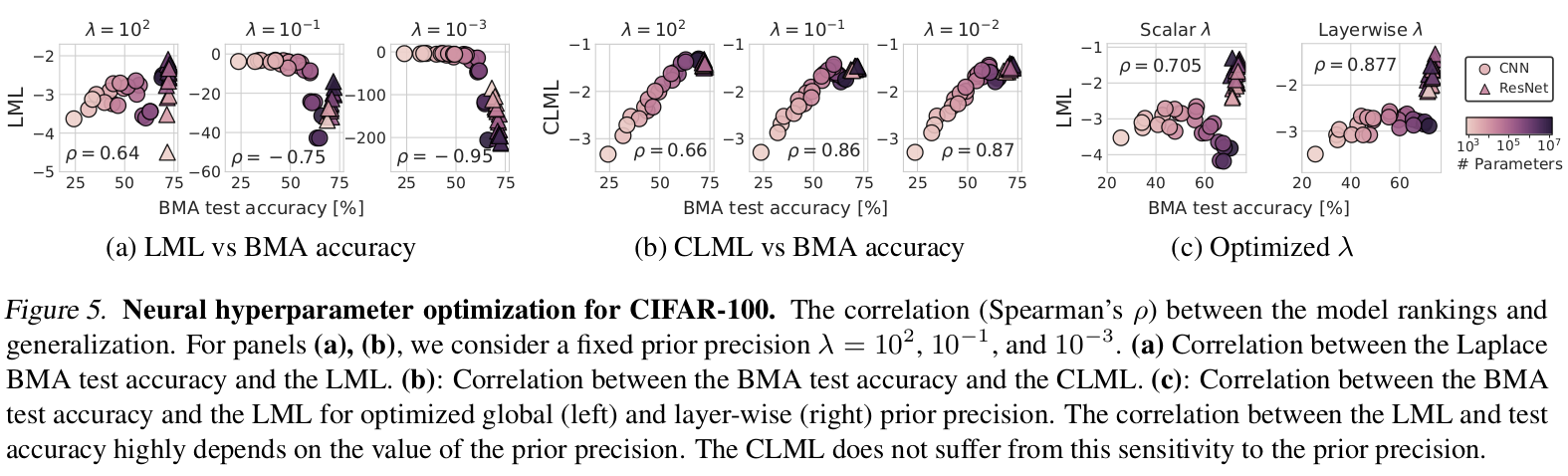
The CLML is more strongly correlated with the generalization performance of the architectures than the LML. The LML suffers from higher first terms in the sum decomposition for more flexible models and is negatively correlated with test accuracy for smaller \(\lambda\). The paper notes that the LML estimate using the LA’s entropy is sensitive to the prior variance and the number of model parameters. This could also explain why larger models have worse LML.
The CLML is computed using predictions on the held-out data for parameter samples from the LA (“function space”), does not estimate the model entropy, and thus does not suffer from the same issues.
Hyperparameter Learning
And?
While the paper covers a lot more in its breadth, the second half mainly focuses on the CLML and examines the question of how the CLML is different from simply using a validation loss. Again, this is not a question directly examined in the paper, but given the prevalence of validation sets, it might be worth asking what the suggested method provides beyond that.
Ignoring Model Priors
First, from a Bayesian point of view, using the model evidence (LML) is only valid for model selection when the model prior is uniform (i.e., all other things are considered equal):
The Bayesian view on model selection given data \(\mathcal{D}\) is: \[ p(\mathcal{M}_i \mid \mathcal{D}) \propto p(\mathcal{D} \mid \mathcal{M}_i) \; p(\mathcal{M}_i). \] Hence, maximizing \(p(\mathcal{D} \mid \mathcal{M}_i)\) is not sufficient depending on what model prior we use.
In particular, the minimum description length (MDL) approach states that we want to select the model that minimizes both the length of describing its parameters and the data.
That is, MDL is about compressing the model and data: \[ \min_i H[\mathcal{M_i}, \mathcal{D}] = \min_i H[\mathcal{D} \mid \mathcal{M_i}] + H[\mathcal{M_i}], \] where \(H\) is Shannon’s information content here (using the Practical IT notation). We can also rewrite this as \[ \begin{aligned} \arg \min_i H[\mathcal{M_i}, \mathcal{D}] &= \arg \min_i H[\mathcal{M_i} \mid \mathcal{D}] + H[\mathcal{D}] \\&= \arg \min_i H[\mathcal{M_i} \mid \mathcal{D}], \end{aligned} \] and we can drop \(H[\mathcal{D}]\) as it is independent of the model.
By ignoring the model complexity when we only use the LML, we might potentially ignore an essential part of Occam’s razor and the MDL principle. However, many other papers also ignore the model complexity and assume a uniform model prior. A uniform prior is valid, for example, when choosing specific hyperparameters. Moreover, estimating a model’s description length is challenging and an open problem. However, the LML only makes sense for model selection when comparing models of equal complexity.
Comparison to Prior Art
We expand on the prior art mentioned in the paper to be able to place it better in the relevant literature.
CLML vs Cross-validation
As noted in the paper, Fong and Holmes (2020)’s “On the marginal likelihood and cross-validation” connects LML and leave-p-out cross-validation:
 = 1 n p ( nXp) t=1 1 p Xp j=1 s y˜ (t) j | y (t) 1:n−p (6) where y˜ (t) 1:p denotes the tth of n-choose-p possible held-out test sets, with y (t) 1:n−p the corresponding training set, such that y1:n = y˜ (t) , y(t) , and SCV records the average predictive score per datum.")
We obtain:
 = Xn p=1 SCV (y1:n; p) (7) with s(˜yj | y1:n−p) = log pM(˜yj | y1:n−p) = log R fθ(˜yj ) dπ(θ | y1:n−p).")
This follows from writing out the terms and swapping the order of the sums.
The paper finally defines something similar to the CLML:
 = X P p=1 SCV (y1:n; p) (8)")
CLML vs TSE-E
While Lyle et al. (2020) focus on the sum under the learning curve as a proxy for the LML, they only note preliminary empirical evidence for a connection to generalization for DNNs. In the follow-up paper “Speedy Performance Estimation for Neural Architecture Search” by Ru et al. (2020), not cited here, the authors focus on using similar ideas for model selection.
In “Speedy Performance Estimation for Neural Architecture Search,” they explain that:
we hypothesise that an estimator of network training speed that assigns higher weights to later epochs may exhibit a better correlation with the true generalisation performance of the final trained network” and evaluate training speed estimators which discount the initial terms and sum over a left-truncated learning curve, amongst others.
The particular estimator is referred to as TSE-E in the paper and shown to have a higher correlation with the generalization performance than the full-length TSE estimator, which is just a proxy for the LML from Lyle et al. (2020). Thus, the findings in this earlier paper are congruent with the CLML.
CLML vs Validation Loss
A different way of examining what the CLML does is to note that the more data a model has trained with, the more its predictions for different samples will become independent. This follows from the model converging to a delta distribution and is, in particular, valid when using a Laplace approximation to the posterior, as is the case here.
In general, we have: \[\begin{aligned} &\log p(\mathcal{D}_{\ge m} \mid \mathcal{D}_{<m}, \mathcal{M}) \\&\quad = \sum_{i=m}^n p(\mathcal{D}_i \mid \mathcal{D}_{<m}, \mathcal{M}) - TC(D_m, \ldots, D_n \mid \mathcal{D}_{<m}, \mathcal{M}), \end{aligned}\] where \(TC(D_m, \ldots, D_n \mid \mathcal{D}_{<m}, \mathcal{M})\) is the total correlation of the samples in \(\mathcal{D}_{\ge m}\) and is thus defined: \[ \begin{aligned} & TC(D_m, \ldots, D_n \mid \mathcal{D}_{<m}, \mathcal{M}) := \\ &\quad = \log p(D_m, \ldots, D_n \mid \mathcal{D}_{<m}, \mathcal{M}) - \sum_{i=n}^m \log p(D_i \mid \mathcal{D}_{<m}, \mathcal{M}). \end{aligned} \]
For \(m→\infty\), we have \(TC(D_m, \ldots, D_n \mid \mathcal{D}_{<m}) \to 0\): The more the model converges, the more the LML is just the cross-entropy of the model trained on \(\mathcal{D}_{<m}\), evaluated on the held-out data times the number of samples in _{m}.
While this might not be true for DNNs overall—deep ensembles that capture multiple modes come to mind—it is true when using a Laplace approximation.
To be precise, the paper always computes the average CLML: it divides the CLML by the number of elements in the \(\mathcal{D}_{\ge m}\). As such, the (negative) validation loss (as negative cross-entropy estimate using the “validation set” \(\mathcal{D}_{\ge m}\)) and average CLML \(\frac{\log p(\mathcal{D}_{\ge m} \mid \mathcal{D}_{<m}, \mathcal{M})}{|\mathcal{D}_{\ge m}|}\) are directly comparable.
In appendix D, the paper explains how many orderings the CLML is averaged over for permutation invariance for the neural architecture experiments on CIFAR-10 & CIFAR-100:
When D is a large dataset such that \(\mathcal{D}_{<m}\) and \(\mathcal{D}_{≥m}\) are both sufficiently large, a single permutation may suffice.
The paper notes that the DNN experiments use an 80%/20% split on CIFAR-10 using only 20 LA samples: A model is trained using 80% of the training data and then evaluated on a 20% held-out “validation set.” The CLML of this model is compared to the (BMA) test accuracy or test (cross-entropy) loss of a model trained on 100% of the training data. The LML is finally estimated using the LA of a model trained on 100% of the training data.
From our recent note “Marginal and Joint Cross-Entropies & Predictives for Online Bayesian Inference, Active Learning, and Active Sampling”, we can hypothesise that 20 LA samples are probably not sufficient to obtain a good CLML estimate (which corresponds to estimating a joint prediction). It is more likely that we only obtain a sample of the validation loss (as sum of marginal predictions) than a good sample of the CLML.
Sadly, the paper does not compare the validation loss and their CLML estimate. The difference between the two quantities would tell us how well the 20 LA samples account for the total correlation.
Laplace Approximation for LML vs Sampling for CLML
There might be an apple vs oranges comparison because the LML is computed using the LA while the CLML is computed via sampling: \[\begin{aligned} \log p(\mathcal D_{\ge m} \mid \mathcal D_{< m}, \mathcal{M} ) &\approx \log \sum_{k=1}^K \frac{1}{K}\, p(\mathcal{D}_{\ge m} \mid w_k, \mathcal M ) \\ &= \log \sum_{k=1}^K \frac{1}{K}\, \prod_{j=m}^n p(y_j \mid x_j, w_i, \mathcal M ), \end{aligned}\] where \(w_k \sim p(\omega_k \mid \mathcal{D}_{<m}, \mathcal M)\) are parameter samples drawn from the LA for the model trained with a subset of the training data (80% of the training data).
Unexpected Anti-Correlation
Previously, we have highlighted the finding from Section 5 that:
correlation of the BMA test log-likelihood with the LML is positive for small datasets and negative for larger datasets, whereas the correlation with the CLML is consistently positive.
Yet, the more data we have, the more the LML should correlate with the final performance simply because the model’s LA will converge, as the following informal reasoning shows:
If we use \(H[Y|X, \mathcal{D}_{\le n}, \mathcal{M}]\) to denote the average cross-entropy (loss) of the model class \(\mathcal M\) when trained on \(\mathcal D _{\le n}\) with \(n\) samples on the test distribution and \(H[\mathcal{D}_{\le n} \mid \mathcal M]\) to denote the (negative) LML, we expect: \[ \frac{H[\mathcal{D}_{\le n} \mid \mathcal M]}{n} \overset{n\to\infty}{\to} H[Y \mid X, \mathcal D _{\infty}, \mathcal M]. \] This is just saying the averaged (negative) LML converges to generalization loss of the model with “optimal” model parameters as we train on more and more data. In particular, the first few terms will matter less and less.
Staying informal (but hopefully still correct), we see that for the correlation coefficient, dividing by \(n\) cancels out: \[ \begin{aligned} &\rho_{\frac{H[\mathcal{D}_{\le n} \mid \mathcal M]}{n} ,\, H[Y \mid X, \mathcal D _{\le n}, \mathcal M]} = \\ &\quad =\frac{Cov[\frac{H[\mathcal{D}_{\le n} \mid \mathcal M]}{n} , H[Y \mid X, \mathcal D _{\le n}, \mathcal M]]}{\sqrt{Var[\frac{H[\mathcal{D}_{\le n} \mid \mathcal M]}{n}] \, Var[ H[Y \mid X, \mathcal D _{\le n}, \mathcal M]]}} \\ & \quad = \frac{Cov[H[\mathcal{D}_{\le n} \mid \mathcal M], H[Y \mid X, \mathcal D _{\le n}, \mathcal M]]}{\sqrt{Var[H[\mathcal{D}_{\le n} \mid \mathcal M]] \, Var[ H[Y \mid X, \mathcal D _{\le n}, \mathcal M]]}} = \\ &\quad = \rho_{H[\mathcal{D}_{\le n} \mid \mathcal M], \, H[Y \mid X, \mathcal D _{\le n}, \mathcal M]} \end{aligned} \] And hence: \[ \rho_{H[\mathcal{D}_{\le n} \mid \mathcal M], \, H[Y \mid X, \mathcal D _{\le n}, \mathcal M]} = \rho_{\frac{H[\mathcal{D}_{\le n} \mid \mathcal M]}{n}, \, H[Y \mid X, \mathcal D _{\le n}, \mathcal M]} \overset{n\to\infty}{\to} 1 \] Given this, LML and generalization loss should correlate positively with sufficient data.
DNN Experiments: Validation Loss vs CLML
Lastly, the initially published DNN experiments in the paper did not compute the CLML but the validation loss. This has been fixed in v2 of the paper.
The logcml_
files in the repository contain the code to compute the CLML for
partially trained models. However, instead of computing \[
\begin{aligned}
\log p(\mathcal D_{\ge m} \mid \mathcal D_{< m}, \mathcal{M} )
\approx \log \sum_{k=1}^K \frac{1}{K}\, p(\mathcal{D}_{\ge m} \mid w_k,
\mathcal M ) \\
= \log \sum_{k=1}^K \frac{1}{K}\, \prod_{j=m}^n p(y_j \mid x_j, w_k,
\mathcal M ),
\end{aligned}
\] the code computes: \[
\begin{aligned}
&\frac{1}{|\mathcal{D}_{\ge m}|}\,\sum_{j=m}^n \log p(\mathcal D_{j}
\mid \mathcal D_{< m}, \mathcal{M} ) \approx \\
&\quad =\frac{1}{|\mathcal{D}_{\ge m}|}\,\sum_{j=m}^n \log
\sum_{k=1}^K \frac{1}{K}\, p(y_j \mid x_j, w_k, \mathcal M ),
\end{aligned}
\] which is the validation cross-entropy loss of the BMA (of the
model trained with 80% of the training data).
**Detailed Code Review**
The high-level [code](https://github.com/Sanaelotfi/Bayesian_model_comparison/tree/c6f0da1d49374c0dda6ee743e5b02bcf3e158e96/Laplace_experiments/cifar/logcml_cifar10_resnets.py#L295) that computes the CLML is:1
2
3
4
5
bma_accuracy, bma_probs, all_ys = get_bma_acc(
net, la, trainloader_test, bma_nsamples,
hessian_structure, temp=best_temp
)
cmll = get_cmll(bma_probs, all_ys, eps=1e-4)
1
2
3
4
5
6
7
8
9
10
11
12
13
14
15
16
17
18
19
20
21
[...]
for sample_params in params:
    sample_probs = []
    all_ys = []
    with torch.no_grad():
        vector_to_parameters(sample_params, net.parameters())
        net.eval()
        for x, y in loader:
            logits = net(x.cuda()).detach().cpu()
            probs = torch.nn.functional.softmax(logits, dim=-1)
            sample_probs.append(probs.detach().cpu().numpy())
            all_ys.append(y.detach().cpu().numpy())
        sample_probs = np.concatenate(sample_probs, axis=0)
        all_ys = np.concatenate(all_ys, axis=0)
        all_probs.append(sample_probs)

all_probs = np.stack(all_probs)
bma_probs = np.mean(all_probs, 0)
bma_accuracy = (np.argmax(bma_probs, axis=-1) == all_ys).mean() * 100

return bma_accuracy, bma_probs, all_ys
1
2
3
4
5
6
7
8
9
10
11
def get_cmll(bma_probs, all_ys, eps=1e-4):
    log_lik = 0
    eps = 1e-4
    for i, label in enumerate(all_ys):
        probs_i = bma_probs[i]
        probs_i += eps
        probs_i[np.argmax(probs_i)] -= eps * len(probs_i)
        log_lik += np.log(probs_i[label]).item()
    cmll = log_lik/len(all_ys)

    return cmll
The DNN experiments in Section 5 and Section 6 of the paper (v1) thus did not estimate the CLML per-se but computed the BMA validation loss of a partially trained model (80%) and find that this correlates positively with the test accuracy and test log-likelihood of the fully trained model (at 100%). This is not surprising because it is well-known that the validation loss of a model trained 80% of the data correlates positively with the test accuracy (and generalization loss).
Conclusion
It would be interesting to determine how the CLML estimated via LA compares with the LML estimated via LA. Similarly, comparing the CLML to the validation loss would be interesting.
However, my expectation is that an estimate via sampling will not be different very different from the validation loss simply because sampling-based approaches do not seem to be working well for estimating joint predictive distributions. This is a finding detailed in our recent note “Marginal and Joint Cross-Entropies & Predictives for Online Bayesian Inference, Active Learning, and Active Sampling”.
Author Response
The following response sadly seems to target the first draft mainly. However, it is also helpful for the final blog post and provides additional context.
Ablation: CLML vs. BMA Validation Loss vs. (non-BMA) Validation Loss
Let us examine the new results:
In the three panels below, two panels show test accuracy vs. validation loss; one shows test accuracy vs. CLML. The left-most panel is the BMA test accuracy vs. (negative) BMA validation loss, the middle panel is vs. the CLML, and the right-most panel is vs. the (negative) non-BMA validation loss.
Note that the left-most panel is from v1, which was accidentally computing the BMA validation loss, and whose axis label I have adapted from v1 for clarity. The two other plots are from v2 after fixing the bug. See commits here for fixing the CLML estimation and here for computing the non-BMA validation loss.


At first glance, there might be an observer effect in the experiments for the validation loss. The BMA validation loss in v1 performs better than the CLML in v2, while the non-BMA validation loss in v2 underperforms the CLML in v2. I asked the authors about it: they pushed the respective code (see link above) and explained that the updated, right-most panel computes the non-BMA validation loss, i.e., without LA samples. To me, it seems surprising that there is such a difference between the non-BMA validation loss and BMA validation loss: the non-BMA validation loss is more than one nat worse on average than the BMA validation loss, based on visual inspection. Note that the plots here and in the paper compute the average CLML and average validation loss and are thus directly comparable.
The authors said in their response that:
You suggest in your post that the validation loss might correlate better with the BMA test accuracy than the CLML given that we use 20 samples for NAS. Our empirical results show the opposite conclusion.
This is only partially true. The BMA validation loss (which was accidentally computed in v1 instead of the CLML) correlates very well with the BMA test accuracy. This is not surprising given that this is the frequentist purpose of using validation sets. If validation sets were not correlating well with the test accuracy, we would not be using them in practice. 🤗 As such, I wonder why the non-BMA validation loss negatively correlates with the BMA test accuracy for ResNets and overall in the v2 results. Thus, only the non-BMA validation loss supports the opposite conclusion in v2 of the paper and in the authors’ response.
Yet what is also surprising is how well the BMA validation loss does vs. the CLML:
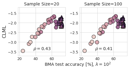
Ablation: LA Sample Size
Secondly, when we compare the reported values between BMA validation loss and CLML, we notice that the CLML is lower than the BMA validation loss by half a nat for \(\lambda=10^2\) and generally for CNNs.
However, it seems, even though the new experiments in v2 are supposed to reproduce the ones from v1, and I assume that the same model checkpoints were used for re-evaluation (as retraining is not necessary), both CLML and non-BMA validation loss are off by about half a nat for the CNNs. As such, the above consideration might hold but might not provide the answer here.
Instead, I have overlaid the non-BMA validation loss and the CLML plots, both from v2, with a “difference blend”: it shows the absolute difference between the colors for overlapping data points (the circles 🔴 and triangles 🔺), leading to black where there is a match, negative (green-ish) color for CLML, and positive (sepia) color for validation losses. I used the background grids to match the plots but hid the ones from CLML afterward—as such, the strong overlay is because the values are so close.

Surprisingly—or rather as predicted when the LA does not really do much—it turns out that the validation loss for the CNNs (🔴) mostly fully matches the estimated CLML with 20 LA samples following a visual inspection. To be more precise, either the models have already sufficiently converged, or the CLML estimate is not actually capturing the correlations between points and thus ends up being very similar to the validation loss.
This changes my interpretation of the sample ablation in the author’s response. The ablation shows no difference between 20 and 100 LA samples, with 100 LA even samples having a slightly lower rank correlation. So it seems x5 more LA samples are not enough to make a difference, or the Laplace posterior cannot capture the posterior as well as we would like. It would be interesting to examine this further. For the previously mentioned note, we have run some toy experiments on MNIST with 10,000 MC Dropout samples previously and did not find good adaptation. Obviously, the LA is not MC Dropout, and this is speculation, but it seems in line with my prior experience.
Recent tweets by @RobertRosenba14 and @stanislavfort also explain why sampling might not be fruitful for estimating joint distributions and compute the CLML in high-dimensional spaces—see here and here.
Given the above, it is fair to say that the estimate of the CLML is probably not as good as hoped, and further experiments might be needed to tease out when the CLML provides more value than the BMA validation loss. Note, however, that this question has not been explicitly examined in the paper. Instead, the paper compares LML and CLML with distinct estimation methods for DNNs.
This note is a part of my paper notes series. You can find more here or follow me on Twitter blackhc.